Jeppe Revall Frisvad Associate Professor in Computer Graphics, M.Sc.(Eng.), Ph.D. Image Section DTU Compute Technical University of Denmark Contact information Home Publications Teaching Code Packages Press Appearances

Interactive Directional Subsurface Scattering and Transport of Emergent Light

Alessandro Dal Corso · Jeppe Revall Frisvad · Jesper Mosegaard · J. Andreas Bærentzen

Abstract Existing techniques for interactive rendering of deformable translucent objects can accurately compute diffuse but not directional subsurface scattering effects. It is currently common practice to gain efficiency by storing maps of transmitted irradiance. This is however not efficient if we need to store elements of irradiance from specific directions. To include changes in subsurface scattering due to changes in the direction of the incident light, we instead sample incident radiance and store scattered radiosity. This enables us to accommodate not only the common distance-based analytical models for subsurface scattering but also directional models. In addition, our method enables easy extraction of virtual point lights for transporting emergent light to the rest of the scene. Our method requires neither preprocessing nor texture parameterization of the translucent objects. To build our maps of scattered radiosity, we progressively render the model from different directions using an importance sampling pattern based on the optical properties of the material. We obtain interactive frame rates, our subsurface scattering results are close to ground truth, and our technique is the first to include interactive transport of emergent light from deformable translucent objects.

Reference

Dal Corso, A., Frisvad, J. R., Mosegaard, J., and Bærentzen, J. A. Interactive directional subsurface scattering and transport of emergent light. The Visual Computer 33(3), pp. 371-383, March 2017. [abstract] [video] [lowres pdf]

Supplementary Appendix on the Directional Dipole Model

To ease implementation of the directional dipole model, we here provide a set of drop-in equations. Notation is explained in the following figure (which is also Fig. 2 in the present publication), and the BSSRDF function $S_d$ given below can be used directly in the theory of the interactive technique.

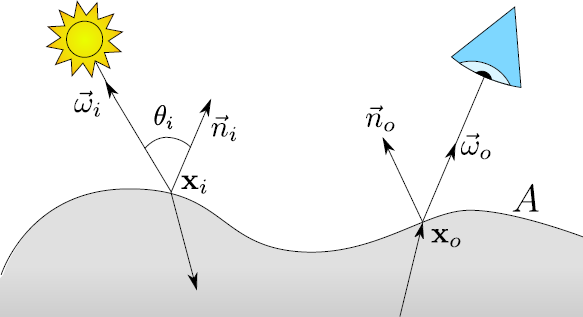Figure. BSSRDF configuration on an object surface $A$. The diagram illustrates the notation
we use: bold font as in $\mathbf{x}_o$ denotes a point, while arrow overline as in $\vec{\omega}_i$ denotes a
normalized direction vector.

As other BSSRDF models, the directional dipole uses a number of inputs that are based on the optical properties of the translucent material ($\eta$, $\sigma_s$, $\sigma_a$, $g$):

\[ \begin{array}{@{}l@{\qquad}l@{\qquad}l@{}} \sigma_t = \sigma_s + \sigma_a \,,& \sigma_s' = (1 - g)\sigma_s \,,& \sigma_t' = \sigma_s' + \sigma_a \,,\\ D = 1/(3\sigma_t') \,,& d_e = 2.131\,D \sqrt{\sigma_t'/\sigma_s'} \,,& \sigma_{\mathrm{tr}} = \sqrt{\sigma_a/D} \,,\\ A = \frac{1 - C_{\mathbf{E}}}{2C_{\phi}} \,,& C_{\phi} = \frac{1}{4}(1 - 2C_1) \,,& C_{\mathbf{E}} = \frac{1}{2}(1 - 3C_2) \,, \end{array} \]

where $C_1$ and $C_2$ are functions of $\eta$ listed in the figure below. The directional dipole formulas for $S_d$ are [Frisvad et al. 2014]:

\[ S_d(\mathbf{x}_i, \vec{\omega}_i; \mathbf{x}_o) = S_d'(\mathbf{x}_o - \mathbf{x}_i, \vec{\omega}_{12}, d_r) - S_d'(\mathbf{x}_o - \mathbf{x}_v, \vec{\omega}_{v}, d_v) \]

and

\[ \begin{array}{@{}l@{}} S_d'(\mathbf{x}, \vec{\omega}_{12}, r) = \\ \frac{1}{4C_{\phi}(1/\eta)}\frac{1}{4\pi^2} \frac{e^{-\sigma_{\mathrm{tr}}r}}{r^3} \Bigg[C_{\phi}(\eta)\left(\frac{r^2}{D} + 3(1 + \sigma_{\mathrm{tr}}r)\,\mathbf{x}\cdot\vec{\omega}_{12}\right) \\ \,\,{}-C_{\mathbf{E}}(\eta)\Bigg(\!3D(1 + \sigma_{\mathrm{tr}}r)\,\vec{\omega}_{12}\cdot\vec{n}_o \\ \,\,{}-\!\left(\!(1 + \sigma_{\mathrm{tr}}r) + 3D \frac{3(1 + \sigma_{\mathrm{tr}}r) + (\sigma_{\mathrm{tr}}r)^2}{r^2} \mathbf{x}\cdot\vec{\omega}_{12}\right)\!\mathbf{x}\cdot\vec{n}_o\!\!\Bigg)\!\Bigg], \end{array} \]

where the various $S_d'$ arguments are based on positions ($\mathbf{x}_i$, $\mathbf{x}_o$), direction of incidence ($\vec{\omega}_i$), and normals ($\vec{n}_i$, $\vec{n}_o$). For the real source, we have

\begin{eqnarray*} \vec{\omega}_{12} & = & \frac{1}{\eta} ((\vec{\omega}_i \cdot \vec{n}_i) \vec{n}_i - \vec{\omega}_i) - \vec{n}_i \sqrt{1 - \frac{1}{\eta^2} (1 - (\vec{\omega}_i \cdot \vec{n}_i)^2)} \\ d_r^2 & = & \!\left\{\begin{array}{@{}l@{}cl@{}}|\mathbf{x}_o - \mathbf{x}_i|^2 + D\mu_0(D\mu_0 - 2d_e\cos\beta) & , & \textrm{for $\mu_0 > 0$} \\[0.8ex] |\mathbf{x}_o - \mathbf{x}_i|^2 + 1/(3\sigma_t)^2 & , & \textrm{otherwise} \end{array} \right. \\ \mu_0 & = & -\vec{n}_o\cdot\vec{\omega}_{12} \\ \cos\beta & = & -\sqrt{\frac{|\mathbf{x}_o - \mathbf{x}_i|^2 - (\mathbf{x}\cdot\vec{\omega}_{12})^2}{|\mathbf{x}_o - \mathbf{x}_i|^2 + d_e^2}} \, , \end{eqnarray*}

and for the virtual source,

\begin{eqnarray*} \mathbf{x}_v & = & \mathbf{x}_i + 2Ad_e\vec{n}_i^{\ast} \\ \vec{\omega}_v & = & \vec{\omega}_{12} - 2(\vec{\omega}_{12}\cdot\vec{n}_i^{\ast})\vec{n}_i^{\ast} \\ \vec{n}_i^{\ast} & = & \!\left\{\begin{array}{@{}l@{}cl} \vec{n}_i & , & \textrm{for $\mathbf{x}_o = \mathbf{x}_i$} \\[0.8ex] \displaystyle \frac{\mathbf{x}_o - \mathbf{x}_i}{|\mathbf{x}_o - \mathbf{x}_i|} \times \frac{\vec{n}_i\times(\mathbf{x}_o - \mathbf{x}_i)}{|\vec{n}_i\times(\mathbf{x}_o - \mathbf{x}_i)|} & , & \textrm{otherwise} \end{array} \right. \end{eqnarray*}

while $d_v$ is as $d_r$ but using $\mathbf{x}_v$ instead of $\mathbf{x}_i$.

\[ \begin{array}{@{}ll@{}} 2C_1 \approx \!\left\{ \begin{array}{@{\!}r@{}c@{\,}l@{}} 0.919317 - 3.4793\eta + 6.75335\eta^2 - 7.80989\eta^3 & & \\[0.9ex] {}+4.98554\eta^4 - 1.36881\eta^5 & , & \eta < 1 \\[1.5ex] -9.23372 + 22.2272\eta - 20.9292\eta^2 + 10.2291\eta^3 & & \\[0.9ex] {}-2.54396\eta^4 + 0.254913\eta^5 & , & \eta \geq 1 \end{array} \right. \\ 3C_2 \approx \!\left\{ \begin{array}{@{\!}r@{}c@{\,}l@{}} 0.828421 - 2.62051\eta + 3.36231\eta^2 - 1.95284\eta^3 & & \\[0.9ex] {}+0.236494\eta^4 + 0.145787\eta^5 & , & \eta < 1 \\[1.7ex] -1641.1 + \frac{135.926}{\eta^3} - \frac{656.175}{\eta^2} + \frac{1376.53}{\eta} + 1213.67\eta & & \\[1.2ex] -568.556\eta^2 + 164.798\eta^3 - 27.0181\eta^4 + 1.91826\eta^5 & , & \eta \geq 1 \end{array} \right. \end{array} \] Figure. Approximate fits for $2C_1$ and $3C_2$ by d'Eon and Irving [2011].